< SED@ Home Page>       < Theory> < Other servers> < History> < Database>


Part 3: Statistical Synthesis Models

Here is a quite large page. I summarize on it the most important aspects related with the IMF sampling. The structure of the page is:
  1. Introduction to Statistics in synthesis models
  2. Statistics
  3. Confidence Limits
  4. Covariance and Diagnostic Diagrams
  5. Bias
Introduction to Statistics in synthesis models
Evolutionary synthesis models have been traditionally used to study the physical properties of unresolved populations, but they should also be able to reproduce the integrated properties of resolved ones. In both cases the discreteness of the stellar populations must be taken into account and model results must be interpreted in a statistical way, i.e. model outputs are a mean value of a probability distribution with an intrinsic dispersion. Such dispersion must be taken into account in the interpretation of the data and it is especially important when the number of observed stars is small (where the definition of small depends on the observable), or in the analysis of surveys.
The origin of such a dispersion is in the very nature of the Initial Mass Function (IMF, c.f. Fig 1) that gives us the probability of obtaining a number of stars in a given mass range. The dispersion arises from the sampling of the IMF from real stellar systems, which is always an incomplete sampling since the number of stars is always finite. If the system under study has a small number of stars, sampling will produce a larger dispersion with respect to the mean value predicted by synthesis models that assume a completely sampled IMF.


Fig. 1: from Cerviño & Mas-Hesse (1994 A&A 284, 749)


From resolved to unresolved stellar populations


In Fig. 2 I show an example of how to go from a resolved stellar population (where, for example, the B-V vs V-K diagram can be obtained) to integrated properties of unresolved systems. Each point corresponds to an individual Monte Carlo simulation of clusters with 1 star in the top panel, and with 10, 100, and 1000 stars in the lower panels. The cicle corresponds to the result of an model that assumes an infinitely populated IMF. The star corresponds to the mean value of the Monte Carlo simulations.

The plot assumes a Salpeter IMF in the mass range 2-120 Mo for a 10 Myr old star forming burst.


Fig. 2: B-V vs V-K
(click on the figure for an enlarge view)

It can be seen that if the system is very small not only the observed values are apart of the value predicted by synthesis models that assume an infinitely populated IMF, but also, the mean value of the sample is biased with respect to the predictions of the models. Also, the dispersion is larger when the number of stars in the clusters are small.

Dispersion is a natural effect of statistics with a small number of stars... Bias is a natural effect when the number of efective sources is small and the considered quantity does not scale linearly with the number/mass of stars (magnitude, colors, ratios...)

... but how to define the term small?


Statistics

Cerviño et al.(2002 A&A 381, 51), based on the original idea from Alberto Buzzoni (1989 ApJS 71, 817), implemented the computation of an effective number of stars, , in their synthesis code. is defined as:

where \mu(L) is the mean value obtained by synthesis models:

with wi the number of stars with initial mass mi, given by the IMF, and li(mi,t) the individual contribution of each star to the observable L. Analogously,


where it is assumed that wi follows a Poisson distribution (they must be always positive and integer numbers) and that there is no correlation among different wi,wj values.

It can be shown that scales with the number of stars in the system, so
it can be used as a definition of the term small.


As an example, the Fig. 3 shows a 3-D plot of the spectral energy distribution and their corresponding values. It also shows the values for some selected ages (0.1, 5.1 and 11.1 Myr). A Salpeter IMF between 2 and 120 Mo is assumed. values range from 0.001 to 0.01 Mo-1 (except for the ionizing flux, which has lower values).
As an example, the output of synthesis models that try to reproduce the spectral energy distribution of a 105 Mo cluster have a relative dispersion between 10 and 3% (i.e. values between 100 and 1000).
Note that in the galactic context, the most massive OB association known, Cygnus OB2 (c.f.Knödlseder 2000 A&A 360, 539) has transformed into stars 1.7 x 10⁴ Mo of gas, assuming the presence of 120 O stars in the association.


Fig. 3: Form Cerviño et al. (2002 A&A 381, 51)


Confidence Limits

A 90% confidence limit (90%CL) is the region that covered by the 90% of the underlying distribution, i.e., the region covered bewteen the an area of 0.05 and 0.95 (assuming that the underlying distribution is normalized to 1). Obviously, the CL interval depends on the underlying distribution.

The effective number of stars, , can be used as an estimation of the underlying distribution of the obseved quantity. In a first order aproximation the confidence intervals can be obtained assuming that the underling distribution is a standar Poisonian distribution defined by , and rescaled to the mean value obtained in the synthesis code

but much more research is needed in this aspect

For example, for quantity L with a effective number (L) and a mean value (L), the CL+(L) value can be obtained in the following way:


--> CL+()

CL+(L) = CL+() x (L) /


And analogously for the CL-(L) tail. Note that the (L) values must be denormalized by the amount of gas transformed into stars

As an example, let me take the Luminosity at 5500 A at 5 Myr for a Instantaneous burst of solar metallicity with standard mass lost rate. Ussing the results from the http://laeff.esa.es/users/mcs/SED/ we have:
L5500= 0.1117E+33 [erg s-1 A-1 Mo-1]
= 0.8358E-03 [Mo-1]
For a cluster where 104 Mo has been transformed into stars in the mass range 2-120 Mo (i.e. 3.4 x 10⁴Mo or 2 x 10⁵ stars in the mass range 0.1-120 for a Salpeter IMF) we have:

<>= 1.117 1036 [erg s-1 Mo-1]
clus= 8.358
For this value of the CL+ is 14.43 and CL- is 4.70, then, the mean value and its 90% CL interval is:
[erg s-1 A-1]


The CL+ -() intervals can been obtained using the Poisson CL formulation given by Gehrels (1986 ApJ 303, 336), or in the address http://members.aol.com/johnp71/confint.html (where a comparison of Poisson and Gassian CL can be obtained).

In general, the Gassian aproximation is a good aproximation for large values. But large depends to the considered CL (i.e. large is larger for a 90%CL than for a 50%CL).


In the Fig. 4 I show the CL obtained with this method (lines) compared with the one obtained from Monte Carlo simulations (shadow area) for clusters with 103, 104 (white) and 105 stars, for V-K (left) and EW(Hbeta) (right).


Fig. 4: Form Cerviño et al. (2002 A&A 381, 51)


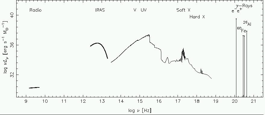
In the Fig. 5 I show the CL obtained with this method for the multiwavelenght energy distribution for Z=0.020; Salpeter IMF, IB, 5.5 Myr, =20%


Fig. 5:    1. Analytical result       2. 105 Mo [2-120 Mo]       3. 104 Mo [2-120 Mo]       3. 103 Mo [2-120 Mo]       5. Comparison
Click on the numbers to see the effect of smapling.


Covariance and Diagnostic Diagrams

For two quantities L1 and L2 it is possible to obtain the covariance using:

equation15

that is related with the correlation coefficient by:

equation22

It can be also demonstrated that tex2html_wrap_inline84 is independent of the sampling. Then it is possible to obtain the confidence levels of the diagnostic diagrams obtained by synthesis models in function of the number of stars (or the mass into stars) in the modeled star forming region.

Note that it is necessary to take into account the dispersion in both axes for the computation of the Confidence Interval in diagnostic diagrams.


Gaussian distributions

In the case of Gaussian distributions, the ellipse:

equation29

gives us the region covered by a Confidence Level CL (As reference, tex2html_wrap_inline86 and tex2html_wrap_inline88 ). In the case that tex2html_wrap_inline90 the ellipse becomes a straight line, and, in other cases, the ellipse is tilted by an angle tex2html_wrap_inline92 given by:

equation42

If tex2html_wrap_inline94 , tex2html_wrap_inline96 (deg) according with the value of tex2html_wrap_inline98 .

Note that tex2html_wrap_inline92 will be always the same whatever the number/mass of stars.

The ellipse semiaxes, a and b are given by:

equation46

equation50

Different cases ares showed in the Figure:
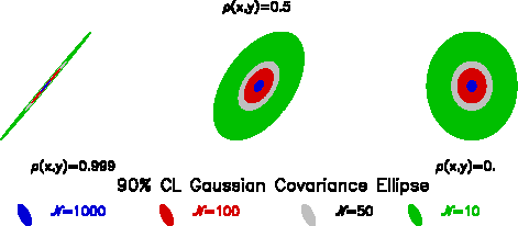
tex2html_wrap136


Quasi-Poisson distributions

The absolute (denormalized) value of tex2html_wrap_inline106 defines the mean value of a quasi-Poisson distribution. In this case, tex2html_wrap_inline108 does NOT correspond to tex2html_wrap_inline110 68% of the full height maximum (i.e. 68% CL) of the underlying distribution, nor tex2html_wrap_inline112 defines the 99% CL (that is the case of Gausanian distributions).

Note also that Gaussian distributions allow the existence of negative values. This occurs when tex2html_wrap_inline114 , but it has NO physical meaning (number of stars, luminosities, intensities, etc... are positive defined quantities) . Then, the Gaussian approximation certainly will fail when tex2html_wrap_inline116 , i.e. tex2html_wrap_inline118

Even more, the underlying distributions are not symmetric and may present different values for the upper (CL+) and the lower (CL-) tails. Also, the region covered by the given CL will not be an ellipse. However such region will be inside the box delimited by tex2html_wrap_inline120 and tex2html_wrap_inline122

So, only in the case of large tex2html_wrap_inline106 values ( tex2html_wrap_inline126 ) the underlying distribution can be approximated by a Gaussian one. To illusitrate this item we compare in the figure the corresponding Gaussian ellipses with the boxes that includes the 90% CL for Poisson distributions:
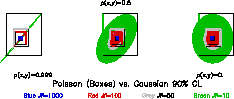
tex2html_wrap138


An example: Results for WR population

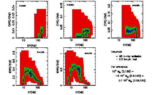
As an example, I show the results for the EW(WR bump) vs. EW(H tex2html_wrap_inline128 ) and I(WR bump)/I(H tex2html_wrap_inline128 ) vs. EW(H tex2html_wrap_inline128 ) diagnostic diagrams in the next figures. A covering factor of 0.7 (i.e. 0.3 of the ionizing photons are lost) is assumed to obtain the I(H tex2html_wrap_inline128 ) emission line and the nebular contribution to the continuum. The simulation does not include the X-ray contribution. Figures make use of Geneva evolutionary tracks with standard mass-loss rates (see astro-ph/0206169) (click in the figure for a better resolution one).
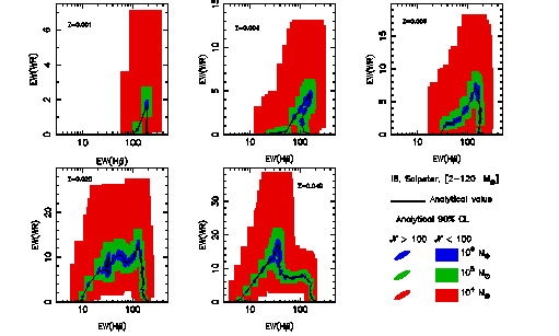


This figures can be compared with the results from Pindao, Schaerer et al. (2002 A&A 394, 443) taken into account that the WRbump here includes all the band and the one computed in that article are only some selected lines in the band (i.e. here the bump is about a factor 3 larger). Comparing the figures you can evaluate how relevant the sampling effects may be...


Bias


The final point to be addressed in this subject is the bias of the results of synthesis models respect to real observations. This bias in related with the Lowest Luminosity Limit quoted before. For a more exaustive reading of the problem I refer to Cerviño, & Valls-Gabaud, (2003 MNRAS 338, 481).


Let me began with with the work of Bruzual (2002; astro-ph/0110245) who show the next figure:
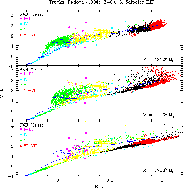


Here the big points corresponds to different clusters with SWB Class (a class defined to stimate the age), the blue line corresponds to the analytical (standard) result and the small dots corresponds to Monte Carlo simulations for different amount of gas transformed into stars (the color code, corresponds to different ages). Note that different colors are overimposed (light bule points are oculted y green points for 104Mo and 103Mo simulations and green points are oculted y yellow points for 103Mo simulations etc..). In his paper he does not talk about the bias of the results of the synthesis models obtained from Monte Carlo simulations (where the number of stars is discrete) and analytical simulations, but such a bias is clear in the figures.

The effect is quite important and general for ratios (like equivalent widths), colors or log quantities. I refer again to Cerviño, & Valls-Gabaud, (2003 MNRAS 338, 481) for a more detailled explanation.


< SED@ Home Page>       < Theory> < Other servers> < History> < Database>